Explaining Variances

As FP&A professionals, we’re tasked with relating the story of the business to the numbers in the P&L. Often, however, the story has many twists and turns that can be hard to break down. Seeing average cost per unit rising drastically over a short period of time can be alarming, but breaking it into the component (i.e. rate, volume, mix, etc.) can help us understand whether the change is a matter of poor management or favorable shift in business volume.

 

One of my favorite ways to present variance analysis is by breaking the variances down to their components – or drivers. For instance, in a manufacturing scenario, your drivers of expense might be wages & benefits, material costs, and hours worked. I’ve broken such a scenario down for you below which can explain the approach.

 

In this scenario, a manufacturer ran production for an order of one of its products

Budget Production Cost		$73,000
Actual Production Cost		$71,100
Cost Higher/(Lower)		($1,900)

 

On the surface, production costs ran slightly lower than budget, but on a per-unit basis, the picture gets much clearer.

Budget Production Cost per Unit (3,500 Units)		$20.86
Actual Production Cost per Unit (2,800 Units)		$25.39
Cost Higher/(Lower)		$4.54

 

Let’s look at the full detail of the production run to see if we can figure out what’s driving the variance to production cost.

 

			Budget		Actual
	Units Produced		3,500		2,800
	Hours per Unit		0.33		0.40
	Burdened Labor Cost		$30.00		$32.50
	Materials Cost per Unit		$8.00		$9.00
	Overhead Costs		$10,000		$9,500
	Total Production Cost		$73,000		$71,100
	Cost per Unit		$20.86		$25.39
	Variable Cost per Unit
	Hours per Unit		0.33		0.40
	Budgeted Labor Cost per Hour		$30.00		$32.50
Labor		$10.00		$13.00
Materials		$8.00		$9.00
			$18.00		$22.00

 

While production costs ran much higher than planned, this chart still doesn’t give us the full picture as to what is driving the incremental expense. The best way to breakdown this variance is to look at the components of the variance starting with the change in volume (i.e. what should the costs have been had we achieved our budgeted variable production cost)?

 

A. Budgeted Units	3,500
B. Actual Units	2,800
C = A - B Difference H/(L)	(700)
D. Budgeted Variable Cost Per Unit	$                18
C. Change in Units Produced	(700)
Variance attributed to change in units produced = C * D	$       (12,600)

All other things being equal, on the budgeted variable cost of $18/unit, producing 700 fewer units should have resulted in $12,600 lower production cost.

 

From here, we can evaluate the variances in different ways, but we’ll need to keep in mind what elements of the variance we’ve already explain as to not explain the same variance driver multiple times. I prefer to find a logic to walk the variance from budget to actual such as “what do I believe is the largest variance driver” or “what appears on the P&L first?” I will caveat that based on how you approach this, you may get different answers to each of the components of variance (more on this later).

 

After explaining the change in units produced, every variance explanation needs to use actual units produced as the basis for calculation. Again, if we break the variances down, we want to avoid explaining the same change multiple times or else we’ll overstate the variance when we add the pieces back together.

 

The next variance I want to explain is how the change in hours per unit impacted the production cost.

 

Change in Hours Per Unit		$         5,600
A. Actual Hours	0.40
B. Budgeted Hours	0.33
C = A - B Difference H/(L)	0.07
D. Actual Units Produced	2,800
E = C * D	187
F. Budgeted Labor Cost per Hour	$30.00
Change in HPU = E * F	$          5,600

 

Where Line C in this section explains the hours worked per unit (seven-tenths of an hour, or about four minutes), note that Line D refers to Actual units produced rather than budgeted units produced. Again, since we’ve already addressed the change from budget to actual units produced, every variance from this point forward should be on actual units produced.

 

I could continue to breakdown this analysis, but I believe these examples should be sufficient to explain the variance breakdown.

 

As previously alluded, you can approach this variance analysis in different ways. For instance, you could begin by calculating the variance in hours per unit against the budgeted units produced and end up with different variance values. The below table shows the difference in variance calculations. Ultimately, the challenge in preparing a variance analysis to this level is that a change in any cost driver will influence all other components of cost.

 

Change in Hours per Unit		$         7,000
Budget HPU	0.33
Actual HPU	0.40
	0.07
Budgeted Units Produced	3,500
Budgeted Labor Cost per Hour	$30.00
Incremental Hours	233.33
Change in Labor Cost		$         3,500
Budgeted Labor Cost	$30.00
Actual Labor Cost	$32.50
	$2.50
Actual HPU	0.40
Budget Units Produced	3,500
Projected Hours Worked	1,400
Change in Material Cost		$         3,500
Budgeted Material Cost per Unit	$8.00
Actual Material Cost per Unit	$9.00
	$1.00
Budgeted Units Produced	3,500
Change in Units Produced		$     (15,400)
Budgeted units Produced	3,500
Actual Units Produced	2,800
	(700)
Actual Variable Cost Per Unit	$22.00
Change in Overhead Cost		$          (500)

 

 

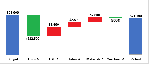
Regardless of how you approach the analysis, we can draw the following conclusions:

1.     The change in units produced is the single largest contributor to the variance

2.     The change in hours per unit erodes much of the cost savings from producing fewer units

 

So, how do you present this analysis? I generally prefer a waterfall chart (which is now available as a stock charting option in Excel). In my experience, visual representation of variances have much more impact on management in helping them to understand the magnitude of change. This method of breaking variances by their drivers allows you to pull out items which might otherwise obscure a significant upside or downside variance.

 

Have you ever used this approach to dive into and explain variances? Outside of manufacturing, what other applications could you apply this methodology to?